Research
Research & Analysis
Full research content from the original portfolio is preserved here: technology and cognitive science, engineering and physics, law and policy, and finance and economics.
Research & Analysis
Technology & Cognitive Science
The Architecture of Cognitive Relief
Why we built a "Life Admin" radar: The psychology of open loops and calm tech.
Read Manifesto +
The Architecture of Cognitive Relief
Why we built a "Life Admin" radar: The psychology of open loops and calm tech.
Read Manifesto +If you constantly feel overwhelmed by the sheer volume of your personal administrative tasks, society has likely given you a misdiagnosis. You’ve probably been told you are lazy, undisciplined, or simply bad at "adulting."
This reductionist view is fundamentally flawed.
The modern citizen has been quietly forced to become their own secretary, compliance officer, IT scheduler, and project manager. We are navigating a highly fragmented digital ecosystem defined by an unprecedented volume of micro-obligations—renewing passports, canceling subscriptions, handling insurance claims, and chasing refunds.
None of these are acute crises in isolation. But collectively, they generate a persistent, invisible cognitive tax. They create "open loops" that run continuously in the background of your mind, severely depleting your cognitive bandwidth.
The software market doesn't need another generic to-do list. The digital landscape is littered with the graveyards of apps that tried to force corporate task-management onto our personal lives. We need a fundamentally different intervention: a system designed explicitly to close mental loops before they metastasize into chronic stress.
We call it Closure. Here is the science of why we built it.
The Psychological Mechanics of "Open Loops"
Attention Residue and the Cost of Context SwitchingThe human brain is biologically ill-equipped for the rapid context switching demanded by modern life. Research by Dr. Sophie Leroy at the University of Washington quantified the severe cognitive penalty of shifting focus. She called it attention residue: the persistence of cognitive activity regarding an unfinished task, even after you’ve stopped working on it.
When you get an email about a housing renewal while you're deep in focused work, you can't complete it instantly. It requires documents you don't have on hand. Because it's left unresolved, it leaves a residue. As you try to return to your work, that open loop continues to siphon your finite mental bandwidth.
The Zeigarnik Effect: The Relief of Plan-MakingHistorically, psychology recognized the Zeigarnik effect: the principle that uncompleted tasks intrude into conscious thought far more than completed ones. It was assumed this background stress would persist until the task was physically done.
But groundbreaking 2011 research by E.J. Masicampo and Roy F. Baumeister changed everything. They proved that you don't actually have to complete a task to get cognitive closure. Allowing subjects to formulate a highly specific, actionable plan completely eliminated the cognitive interference. Formulating a plan signals to your brain's executive functioning center that the matter is handled, allowing the anxiety to cease. Closure is an automated engine for this exact psychological phenomenon.
The Sociological Reality of "Life Admin"
Administrative burden isn't just annoying; it is a systemic issue that extracts a massive toll. A 2022 UK study revealed that everyday administrative tasks consume an average of one full hour per day for the typical adult. This burden breaks down into three distinct costs:
- Learning Costs: The mental effort required to decode complex, opaque instructions.
- Compliance Costs: The friction of gathering documents, proving your status, or navigating bureaucracy.
- Psychological Costs: The acute stress, loss of autonomy, and anxiety of navigating these systems.
Crucially, this workload is often invisible, particularly in households. Harvard researcher Allison Daminger defines cognitive labor as the unseen, continuous mental work required to anticipate household needs. This invisible load disproportionately falls on women, leading to severe burnout and relationship friction. Closure is designed to make this invisible load visible, providing a neutral, shared system to delegate household tasks without turning your relationship into an adversarial corporate environment.
The Antithesis of Calm: Why Current Apps Fail
If the market is saturated with productivity apps, why are we more exhausted than ever? Because current software relies on mechanics that actively harm our mental state.
- The Neurological Assault of Notifications: Standard apps rely on push notifications. A 2022 electrophysiological study definitively proved that processing smartphone notification sounds forces the brain to recruit significantly higher levels of cognitive control, rapidly draining mental energy. When your to-do app pings you with "Reminder: housing thing," it acts as a hostile interruption.
- The "Jira-fication" of Personal Life: Apps optimized for corporate engineering sprints (endless backlogs, complex tagging, color-coded urgency) induce "productivity guilt." They frame rest as a personal failure to clear the backlog.
How Closure Works: Calm Technology in Action
We built Closure on the principles of Calm Technology—systems that work in quiet harmony with human attention rather than exploiting it. The core metric of Closure is not how much time you spend in the app. In fact, if the app works perfectly, your engagement time should plummet. Here is how the architecture is designed to give you your brain back:
You encounter an administrative stressor (e.g., an email stating: "Submit housing documents by June 3"). Without thinking, you simply forward it, text it, or screenshot it directly to Closure.
Our AI backend processes the unstructured data and converts it into an exact next physical action. Instead of "handle housing," it dictates: Upload ID copy and proof of payment (Estimated time: 12 mins).
The system calculates a buffer. Instead of reminding you on the final deadline of June 3, it establishes a "Do before" date of May 29, and issues a strict Safe-until guarantee of May 27. You are explicitly granted psychological permission to stop thinking about the task until May 27.
When it is time to act, the system provides one-tap contextual help, such as a pre-drafted email asking the housing office what constitutes valid proof of payment, lowering your learning cost to near zero.
Privacy as the Ultimate Feature
Because Closure acts as an external brain for highly consequential tasks—medical appointments, financial deadlines, legal documentation—our ethical stance must be unassailable.
If you harbor even a slight suspicion that your intimate data is being mined or sold, the app becomes a source of anxiety, defeating its entire purpose. Therefore, our business model is simple: Zero ads. Zero data brokering. Aggressive data minimization. We discard or heavily encrypt the source material immediately after processing it. We monetize through direct user subscriptions, because when the cost of a missed legal deadline is catastrophic, peace of mind is worth paying for.
The New Standard
You are not lacking discipline. You are carrying too much. Closure is not an application designed to help you do more; it is a vital psychological intervention designed to help you carry less. It is time to return to the profound feeling of: "I am not forgetting anything important."
© Jongpyo Hong
Morning Brief
A browser-based briefing system for organizing the day before the day organizes you.
Engineering & Physics
Impact of applied external resistor and pulse variance in Te-based Ovonic Threshold Switching (SOM)
Simplified Explanation
"How does a material remember the electric pulses it has experienced before?"
Most computers separate memory (storage) and logic (processing). My research explores Selector-Only Memory (SOM), where a material acts like a "smart bouncer"—deciding whether to let current pass based on the history of previous electrical pulses.
By controlling the "rhythm" of these pulses (timing) and the "pressure" (resistance), we can teach the material to remember binary states (0 or 1) without traditional transistors. In short: timing writes history.
Read Full Technical Paper
Jongpyo Hong (2022199013)¹, Siwon Park², Su-Bong Lee², Young-Min Kim², Sangyeop Kim², and Jong-Souk Yeo (advisor)¹²
1. Nano Science and Engineering, Integrated Science and Engineering Division, Underwood International College, Yonsei University
2. School of Integrated Technology, College of Computing Yonsei University
jongsoukyeo@yonsei.ac.kr
Abstract
The integration of phase change memory (PCM) with ovonic threshold switching (OTS) selectors in a 3D crosspoint array has gained attention for its potential and its promising developments in memory technology. Stability and scalability of the integration of PCM with OTS remain a challenge, particularly due to the instability in the threshold voltage of OTS devices from the application of pulses. This research capitalizes on the instability of the threshold voltage and investigates the impact of pulse rise and fall time and external resistor on threshold voltage shift in a Te-based OTS device to enhance the read window margin (RWM), which is a crucial component to realize a reliable binary data storage in selector-only memory (SOM) applications. By varying pulse durations, this research demonstrates that shorter pulses show greater shifts in threshold voltage. This research also demonstrates that addition of higher resistance with external resistors increases the magnitude of both positive and negative threshold voltage shifts. These findings provide a pathway to optimizing OTS devices for better distinction between binary states, thereby enhancing memory reliability for SOM applications.
1. Introduction
Computers have become an indispensable part of our lives, handling from the most mundane tasks to the most demanding, specialized calculations. As the higher end of the spectrum became ever more challenging, especially with today’s furor with artificial intelligence (AI), the search for better memory that meets the requirements including, but not limited to, larger data storage, faster operating speed, better endurance, and greater density has become imperative [1]. The physical segregation of processor and memory units in the traditional von Neumann architecture heavily restricts the amount of data that can be transferred, a phenomenon known as the von Neumann bottleneck [2]. Not only that, but also the traditional charge-based memory devices have low scalability and are power inefficient [3]–[6].
The advent of 3D-stacking memory technology was a step toward satiating the greater density requirement. Employing phase change memory (PCM) cells in a cross-point architecture showed promising results in terms of endurance and scalability [7]. PCM, one of the resistive switching materials (RSMs) that takes advantage of phase transitions between amorphous and crystalline states that exhibit significantly different electrical resistance [2], secured its spot among the numerous candidates for revolutionizing memory.
The highly dense 3D crossbar architecture comes at a cost, however. Word and bit lines can be visualized as skew lines on parallel planes that are connected by the two opposite terminals of a single cell. The word and bit line to which the cell is connected are selected to select a target PCM cell. Since multiple cells belong to either the selected word line or bit line, these cells are half-selected, forming sneak currents [8] that could further entail system failure [9]. Something that selectively allows current to the target cell while suppressing sneak current in others was necessary.
Enter the ovonic threshold switching (OTS) selectors, chalcogenide-based materials that exhibit high electrical resistance below the threshold voltage and low electrical resistance above the threshold voltage. This makes it possible to apply a voltage to the word and bit line of the target memory cell so that the applied voltage to the target cell is above the threshold voltage while the half-selected cells receive less than the threshold voltage. Hence only the target memory cell is selected while the other half-selected cells have negligible current. The combination of PCM cells with OTS selectors in the 3D crosspoint array is thus vital.
However, this method of employing PCM with an OTS selector has problems of its own. The integration of the two different layers of PCM and OTS makes the fabrication process difficult, and the scaled distance between cells further worsens the thermal issues of PCM [11]. Although a selector is needed for PCM to function properly, the stack must be simplified further. Additionally, the threshold voltage of the OTS device is unstable, being noticeably influenced by the pulse applied. Previous studies have reported that an OTS selector exhibits a shift in its threshold voltage as a response to a change in the width, amplitude, ramp rate, and polarity of the pulse [12]–[15].
The shift in the threshold voltage induced by the polarity of the applied pulse, initially considered an undesirable instability, can be capitalized upon to simplify the PCM-OTS stack by using only the OTS device as a memory device without the PCM, creating a selector-only memory (SOM) device. The disparity between the subsequent threshold voltages due to the polarity-induced threshold voltage shift can be utilized to store and retrieve memory. Specifically, a pulse with a value between the two threshold voltages can be applied, and depending on the previously applied pulse, the resulting current will vary: if the pulse is higher than the threshold, there will be a significant current, and if the pulse is lower than the threshold, there will be negligible current. This measurement of resulting current will help ascertain whether the threshold voltage is high or low, which represent the binary values of 0 and 1.
The use of a pulse between the threshold voltage values necessitates that the read window margin (RWM), the difference between the high threshold voltage and the low threshold voltage, be as wide as possible. A greater shift in the threshold voltage is desired as it would allow a clearer distinction between the binary 0 and 1 and hence less prone to errors. Therefore, this research seeks to address the need to enlarge the RWM by modulating the applied pulse. An external resistor was added to the device to alleviate the stress applied to the device by sudden increases in current, and it was observed that resistance also affects the change in threshold voltage. This paper thus investigates the effect of pulse rise and fall time and an external resistor on the change in threshold voltage.
2. Methods
A previous research study discovered that Se-based OTS exhibits a strong polarity effect [16]. Although it showed a strong polarity effect, there are some disadvantages to using Se, including its toxicity [17]. The low melting point of Se also hinders its use as an ideal sputter target, complicating the fabrication process. Therefore, this research selected Te as a substitute for Se because of its expected similar properties for they belong to the same group.
After cleaning the prepared SiO2 wafer with acetone, isopropyl alcohol (IPA), and deionized (DI) water, a bottom electrode of Tungsten is deposited via PVD. SiO2 layer is deposited again on the W layer via CVD, and a photoresist is spin-coated on the topmost layer. After eliminating the desired portions via maskless photolithography, the selected portions of SiO2 are etched via ICP-RIE. After removing the photoresist, the photolithography process is repeated on the device. The OTS material is deposited onto the topmost layer via RF sputter, and after the top electrode of W is sputtered, the photoresist is removed. The bottom electrode and the top electrode are connected to the electrical probes when analyzing the electrical properties of the device.
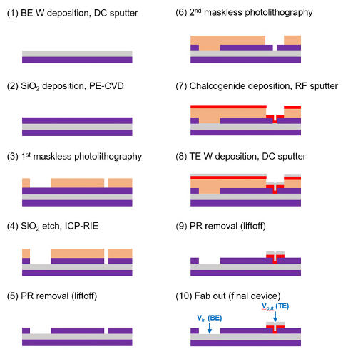
Fig. 1 Fabrication steps of the Te-based OTS devices.
This paper focuses on NSiTe device. Fig. 2 depicts the simple model of the final product of the fabricated device. Using this device, the pulse rise and fall times were initially varied, and the effect on the magnitude of threshold voltage shift was measured. Next, the external resistor applied to the system was varied, and its effect on the threshold voltage shift was also measured.
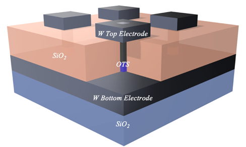
Fig. 2 Final product of the fabricated device.
3. Results and Discussion
3.1. Polarity Effect in Device and Suitable SchemeNSiTe, fabricated via the aforementioned RF co-sputtering process, exhibited a good general trend of polarity-induced threshold voltage shift. It is notable that the direction of the shift is different from the phenomenon referred to in a previous study: the aforementioned polarity effect described a decrease in the threshold voltage for same subsequent polarity pulses and an increase in the threshold voltage for opposite subsequent polarity pulses [15]. NSiTe analyzed in this research, however, exhibited an increase in the threshold voltage for the same subsequent polarity pulses and a decrease in the threshold voltage for the opposite subsequent polarity pulses.
This paper follows the convention of the threshold voltage shift as shown in Equation (1).
The superscript “opp” and “same” refer to the relative polarity of the read pulse to the previous write pulse. Therefore, Equation (1) can be further specified into two separate regions of the negative and positive branches, depicted in Equation (2) and (3).
$$\Delta V_{th}^{\mathrm{POS}} = \left| V_{th,\mathrm{NEG}}^{\mathrm{POS}} \right| - \left| V_{th,\mathrm{POS}}^{\mathrm{POS}} \right|$$
$$\Delta V_{th}^{\mathrm{NEG}} = \left| V_{th,\mathrm{POS}}^{\mathrm{NEG}} \right| - \left| V_{th,\mathrm{NEG}}^{\mathrm{NEG}} \right|$$
The superscript is the polarity of the read pulse, and the subscript is the polarity of the previous write pulse. Since the device of focus in this research generally showed an increase in threshold voltage from subsequent positive pulse and a decrease in the absolute value of threshold voltage from subsequent negative pulse, \( \left| V_{th,\mathrm{POS}}^{\mathrm{POS}} \right| \) is greater than \( \left| V_{th,\mathrm{NEG}}^{\mathrm{POS}} \right| \), and \( \left| V_{th,\mathrm{NEG}}^{\mathrm{NEG}} \right| \) is less than \( \left| V_{th,\mathrm{POS}}^{\mathrm{NEG}} \right| \), and hence, \( \Delta V_{th}^{\mathrm{POS}} < 0 \) and \( \Delta V_{th}^{\mathrm{NEG}} > 0 \).
Devices that showed SOM characteristics in previous studies have generally shown a decrease in the threshold voltage when the write and read pulses are of the same polarity and an increase in the threshold voltage when they are of opposite polarity [16]. Therefore, the application of the device to practical memory uses the following scheme depicted in Fig. 3: when there is no initial write pulse, the read pulse will be the first pulse applied. This read pulse will be lower than the high threshold voltage, so there will be negligible current. This negligible current is translated to binary value of 0, meaning no data is stored. If there was an initial write pulse, the write pulse sets the high threshold voltage. The following read pulse will decrease the threshold voltage. This read pulse is higher than the lower threshold voltage, so there will be significant current. This high current is translated to binary value of 1, meaning data was stored. A reset pulse in the opposite negative direction is applied, and the cycle continues.
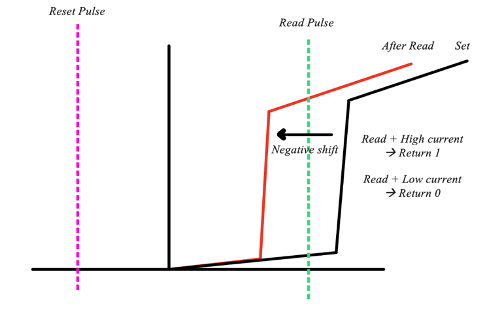
Fig. 3 Scheme for application of previously studied OTS devices for SOM use.
The NST device of this research, however, exhibits a different polarity-induced threshold voltage shift: the threshold voltage increases when the write and read pulses are of the same polarity. Fig. 4 shows the increase in the threshold voltage from the first black pulse to the next red pulse. Therefore, the application of this device requires a new scheme depicted in Fig. 5. If there was no write pulse, the first pulse applied will be the read pulse. This read pulse will set a low threshold voltage, and since this read pulse is higher than the low threshold voltage, there will be significant current. This significant current is translated to binary value of 0, meaning no data is stored. On the other hand, if there was a write pulse, the low threshold voltage will be set initially. The following read pulse will increase the threshold voltage. Since this threshold voltage is higher than the read pulse, there will be negligible current. This negligible current is translated to binary value of 1, meaning that there is data stored. A reset pulse in the opposite negative direction is applied, and the cycle continues.
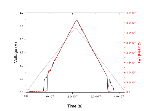
Fig. 4 Threshold voltage shift in positive branch.
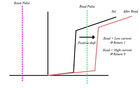
Fig. 5 Scheme for application of NSiTe device.
To explore the different responses of the device to different stimuli, the rise and fall time of pulse applied was first varied into 1, 2, 4, and 8microseconds. However, the input voltage values showed a distinct kink that represents an overshoot due to sudden surge of uncontrolled signal when the switching takes place. This kink hinders accurate reading of the threshold voltage and represented the wearing of the device due to the stress applied by the sudden increase in current. To eliminate this kink and mitigate the stress on the device, an external resistor of 330 ohms was added to the device.
With the external resistor fixed at 330 ohms, the rise and fall time of the applied pulse was again varied. Fig. 6 shows the change in the magnitude of the threshold voltage shift in the positive and negative branches as the pulse rise and fall time is varied. In both the positive and negative branch, the magnitude of the threshold voltage shift decreases as pulse rise and fall time increases. Therefore, to increase the RWM, shorter pulse rise and fall time should be chosen.
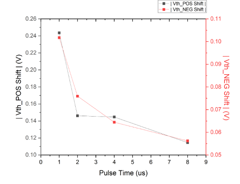
Fig. 6 Change in magnitude of threshold voltage shift.
It should be noted that there were no significant SOM characteristics exhibited by the device when a pulse time of nanoseconds was applied. It was at the microsecond regime in which the device began to show SOM characteristics. Therefore, a shorter pulse time in the microsecond regime should be chosen to optimize for SOM performance. The disparity between nanosecond regime and microsecond regime suggests that sufficient time is needed for a physical change to take place within the device. Perhaps ion migration, with their masses greater than mass of electrons, may be responsible for the longer pulse time required to observe SOM characteristics.
To observe why longer pulse rise and fall time leads to a decrease in the threshold voltage shift, the change in temperature from the different pulse times were compared to observe the effect of Joule heating. Using the applied voltage and current, power could be retrieved by Equation (4).
The power could be used to retrieve energy applied to the device by Equation (5).
Since the specific heat capacity of the device is not known, proportionality Equation (6) of energy to the change in temperature is used.
From these equations, the ratio of the change in temperatures for the pulse rise and fall time of \(1\ \mu s:2\ \mu s:4\ \mu s:8\ \mu s\) is \(62K:91K:236K:468K\), indicating that an increase in pulse rise and fall time leads to an increase in Joule heating effect. This increase in Joule heating may facilitate atomic migration [16], decreasing the threshold voltage and thereby decreasing the scope for change in the threshold voltage, which is measured as the change in the threshold voltage. Ravsher et al. noted that Joule heating in the high operating current regime may confirm the presence of atomic segregation [16], and the NSiTe device operating in the similar high operating current regime (»4 mA) seems to follow this previous study’s observation.
The extent of the change in threshold voltage can be further analyzed by observing percent changes from 1 to 2microseconds, 2 to 4microseconds, and 4 to 8microseconds. The percent change of threshold voltage shift and the percent change in temperature change can be compared to determine whether the changes parallel each other. As pulse time increased, the percent changes in change in temperature were 46.77%, 159.34%, and 98.31%. The percent change in the threshold voltage shifts in positive and negative branches were -40.01%, -0.97%, and -20.82%, and -25.35%, -15.11%, and -12.77%, respectively. The extent of temperature increase seems to generally increase as pulse time increases, but the extent of threshold voltage shift decreases. Assuming ion migration, as the rate of temperature change increases, the rate of threshold voltage shift should increase, but this is not the case as shown in percent changes. This may be due to the ion aggregation over same subsequent polarity pulses that exerts force on other ions in the opposite direction, making it more difficult for ions to migrate to conduct current. Hence, these aggregated ions may partially counteract the decrease in the threshold voltage, which is exhibited by the decreasing rate of threshold voltage shift. By applying the opposite reset pulse, the aggregated ions may return to their original locations either partially or completely, allowing the device to go through the cycle again.
3.3. Impact of External Resistor on Vth ShiftWhile varying the external resistor to eliminate the kink, differences in the threshold voltage shifts were observed. To explore more on the effect of external resistors on the polarity effect, various resistors that range from 110 ohms to 680 ohms were applied and measured. As shown in Fig. 7 (listed as Fig. 8 in text), the magnitude of threshold voltage shift in both the positive and negative branches increase as the resistance of the applied external resistor increases. Therefore, the application of an external resistor with higher resistance seems to be a better selection to achieve a greater RWM.
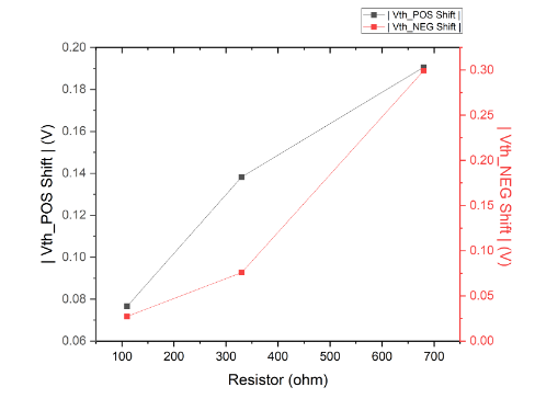
Fig. 7 Change in threshold voltage shift vs external resistor.
This disparity in the magnitude of the threshold voltage shift may also be explained by Joule heating effect. Joule heating is generated due to large current passing through the device as stated by Ravsher et al. [16]. The current that flows through the device with 680 ohms resistor (»2 mA) is still within the high operating current regime [16], indicating that Joule heating may still be sufficient to assist ion migration. Using the same set of Equations (4), (5), and (6), the ratio of the change in temperature for the external resistor of 110W: 330W:680W is 145K:91K:53K, indicating that an increase in resistance of the external resistor leads to a decrease in Joule heating effect. This decrease in Joule heating may decrease the extent of heat-assisted ion migration, increasing the threshold voltage. As the threshold voltage increases, the scope for change in the threshold voltage increases.
3.4 Future WorksTo fully utilize the OTS devices for SOM applications, the threshold voltage must return to the initial threshold voltage after a full cycle (PNN or NPP sequence). The focus then shifts from increasing the RWM to stabilizing the threshold voltage value after applying the same sequence numerous times. Instead of utilizing write and read voltage solely to write and read, additional pulses may be applied after reading and before resetting the device (i.e., instead of PNNPNN, apply PNN…NPNN…N) may further optimize the stability of the set threshold voltage for SOM applications.
4. Conclusion
This study delves into the effects of pulse rise and fall time and external resistance on the shift in threshold voltage in NSiTe ovonic threshold switch (OTS) device. It highlights their significance for enhancing the read window margin (RWM) in selector-only memory (SOM) applications. The experimental results present a clear trend: decreasing pulse time leads to a greater threshold voltage shift, and increasing resistance of the external resistor leads to a more pronounced shift. Several factors including controlled current flow and resulting Joule heating effect are proposed as responsible for these shifting behaviors.
The findings highlight the crucial role of pulse time and external resistors in increasing RWM to improve the distinction between binary states and reducing error rates in memory operations. This research contributes insights into the optimization of OTS-based memory systems, paving the way for more robust yet simplified SOM solutions.
Future works should focus on further increasing the threshold voltage shift and stabilizing the set threshold voltage after repetitive cycle of set and reset pulses for practical use of SOM devices. Moreover, investigating long-term reliability and endurance of these devices will be essential for their practical implementation as SOM devices.
5. References
- Zhu, Min & Ren, Kun & Song, Zhitang. (2019). Ovonic threshold switching selectors for three-dimensional stackable phase-change memory. MRS Bulletin. 44. 715-720.
- Wang, Zhongrui et al. (2020). Resistive switching materials for information processing. Nature Reviews Materials. 5. 1-23.
- Waser, Rainer & AONO, MASAKAZU. (2009). Nanoionics-based resistive switching memories.
- Lee, Myoung-Jae et al. (2011). A Fast, High-Endurance and Scalable Non-Volatile Memory Device Made from Asymmetric Ta2O5−X/TaO2−X Bilayer Structures. Nature materials.
- Yang, Jianhua Joshua et al. (2010). High switching endurance in TaOx memristive devices. Applied Physics Letters. 97. 232102.
- Miao, Feng et al. (2011). Anatomy of a Nanoscale Conduction Channel Reveals the Mechanism of a High-Performance Memristor. Advanced materials. 23. 5633-40.
- Lai, S. (2009). Non-Volatile memory technologies: The quest for ever lower cost. IEDM Tech. Dig. 1 - 6.
- Burr, Geoffrey et al. (2014). Access devices for 3D crosspoint memory. Journal of vacuum science & technology B. 32. 040802.
- Park, Chaebin. (2023). Toward Scalable and Sustainable Selector: Ovonic Threshold Switching N-Si-Ge-Te Chalcogenide Selector for 3D Crossbar Neuromorphic Applications [Master’s thesis]. Yonsei University.
- Lee, Jangseop et al. (2023). Enhancing Se-based Selector-only Memory with Ultra-fast Write Speed (~ 10 ns)...
- Hong, Seokman et al. (2022). Extremely high performance, high density 20nm self-selecting cross-point memory...
- Ban, Sanghyun et al. (2020). Pulse Dependent Threshold Voltage Variation of the Ovonic Threshold Switch...
- Ravsher, Taras et al. (2021). Polarity-dependent threshold voltage shift in ovonic threshold switches...
- Chai, Zheng et al. (2019). Dependence of switching probability on operation conditions in GexSe1-x...
- Ravsher, Taras et al. (2023). Self-Rectifying Memory Cell Based on SiGeAsSe Ovonic Threshold Switch...
- Ravsher, Taras et al. (2023). Polarity‐Induced Threshold Voltage Shift in Ovonic Threshold Switching...
- Hamilton, Steven. (2004). Review of selenium toxicity in the aquatic food chain. The Science of the Total Environment. 326. 1-31.
Mathematical Modeling
Kinematics of a Bus: Deriving Safety Margins
Deriving the underlying geometry of a 12m bus lane change.
Kinematics of a Bus: Deriving Safety Margins
Deriving the underlying geometry of a 12m bus lane change.
I. Minimum Clearance for Lane Change
Q: What is the minimum distance to the vehicle in front to avoid scraping during a full-lock lane change?
- Rigid 12m city bus (Single-lane lateral shift)
- Wheelbase (L) = 6.0 m
- Max steering angle (θ) = 40°
- Lane width (w) = 3.50 m
Turning Radius (R):
R = L / tan(θ) = 7.15 m
Forward Advance (x):
φ = arccos(1 - w/R) ≈ 59.3°
x = R sin(φ) ≈ 6.15 m
Result: Adding a 0.5m safety pad, the minimum gap is 6.5 - 7.0 meters. If the driver waits until the rear bumper of the car ahead is 7m clear, the nose will not overlap.
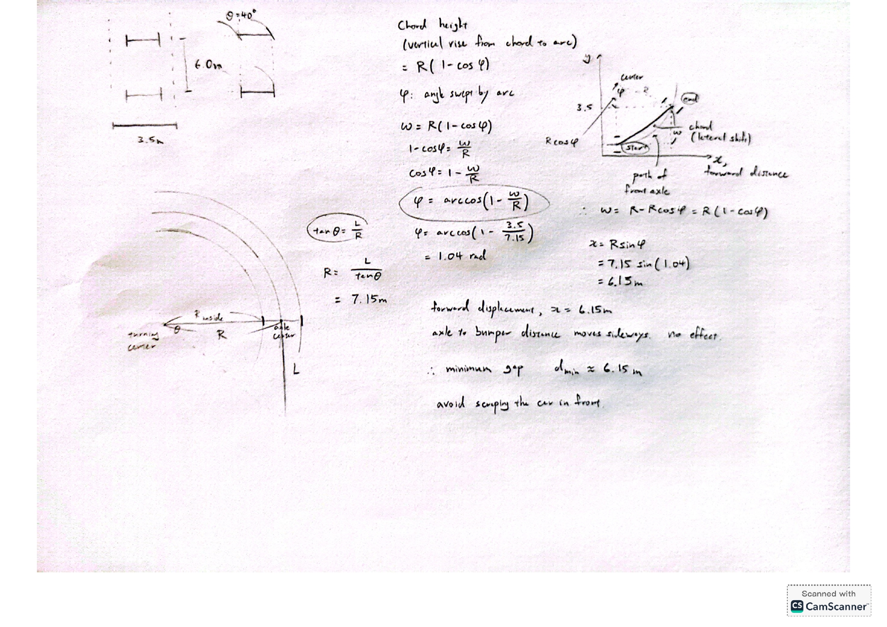
Figure 1: Clearance geometry analysis.
II. The S-Curve Maneuver
Q: How far must the bus run straight before counter-steering to center in Lane 2?
- Full-Left Lock: Enter Lane 2.
- Straight Segment (S): Slide diagonally holding heading +φ.
- Full-Right Lock: Cancel heading to finish centered.
Total Lateral Shift Equation:
yfinal = R(1 - cosφ) + S sinφ + R sin²φ - R(1 - cosφ)cosφ = wlane
Solving for Straight Segment (S):
S = (wlane - R(1 - cosφ)² - R sin²φ) / sinφ
Result: For a half-width shift (1.25m), the bus must roll straight (yawed 34°) for approximately 1.8 meters before counter-steering.
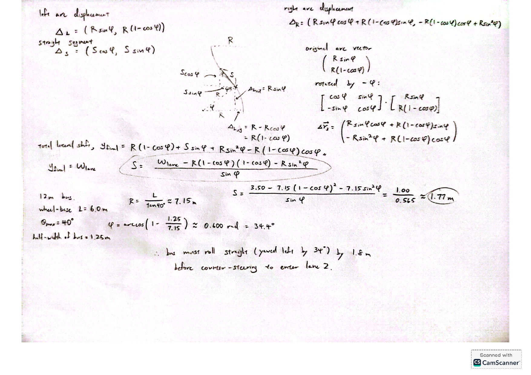
Figure 1: Clearance geometry analysis.
Derivations in Quantum Mechanics
Original handwritten derivations: Complex Analysis to Multi-Qubit Systems.
View PDF
History & Theory
Quantum Einstein, Bohr, and the Great Debate
Notes on the history of the quantum revolution & mathematical derivations.
Quantum Einstein, Bohr, and the Great Debate
Notes on the history of the quantum revolution & mathematical derivations.
I. The Discovery of the Nucleus
- Rontgen (1895): Discovered X-rays ("I did not think; I investigated").
- Becquerel & Curie: Discovered radioactivity; realized it was an atomic phenomenon.
- Rutherford's Gold Foil: Alpha particles fired at gold foil. Most passed through, but some bounced back. Conclusion: Atoms have a tiny, dense, positive nucleus.
II. The Quantum Atom (Bohr)
Problem: Classical physics says orbiting electrons should radiate energy and crash into the nucleus.
Bohr's Solution: "Stationary States." Electrons only occupy orbits where angular momentum is quantized.
1. Quantization Condition:
L = mevr = nℏ
2. Centripetal Force = Coulomb Force:
mev2/r = e2 / (4πε0r2)
3. Solving for Energy (En):
En = -13.6 eV / n2
Result: Explains the discrete spectral lines (Lyman, Balmer) of Hydrogen.
III. Wave-Particle Duality
X-rays colliding with electrons lose energy (wavelength increases). Proves light behaves as a particle (photon).
If waves act like particles, particles act like waves. Electrons form "standing waves" around the nucleus.
IV. The Quantum Magicians
- Heisenberg: Abandoned unobservable "orbits." Developed Matrix Mechanics based only on observable spectral frequencies.
- Pauli: Exclusion Principle. Introduced "Spin" (4th quantum number) to explain the Zeeman effect (splitting of spectral lines in magnetic fields).
- Schrödinger: Developed the Wave Equation (Ψ) to describe probability density.
- Born's Postulate: The square of the wavefunction |Ψ|2 represents the probability of finding a particle.
Law & Policy
Resolving Gödel’s Constitutional Loophole
A proposal to safeguard the Amendment Process against self-destruction.
Read Full Essay +
Resolving Gödel’s Constitutional Loophole
A proposal to safeguard the Amendment Process against self-destruction.
Read Full Essay +Introduction
In 1947, the logician Kurt Gödel famously claimed to have found a loophole in the United States Constitution that could allow the nation to legally transform into a dictatorship. During his U.S. citizenship exam, Gödel told a judge that “this [dictatorship] could not happen in the U.S.” under the Constitution—and then insisted, “Oh, yes, I can prove it,” before being hastily cut off. This mysterious “Gödel’s Loophole” has since been called “one of the great unsolved problems of constitutional law.”
In essence, Gödel had identified a self-referential flaw: an “inner contradiction” in the Constitution’s own amendment rules. The Constitution’s Article V prescribes how it can be amended, but—as Gödel noted—those rules can be used on themselves, potentially undermining any limits to change. This paper examines the nature of Gödel’s loophole and proposes a resolution to safeguard the Constitution’s core principles from self-destructive amendments.
The Self-Amendment Paradox
Article V of the U.S. Constitution outlines a strict process for amendments (requiring supermajority approval by Congress and the states). Gödel’s insight was that Article V can be amended by its own procedure, allowing a downward spiral of ever-easier changes. In other words, one could legally amend Article V to loosen the requirements for future amendments, then amend it again even more easily, and so on. Ultimately, nothing in the text would stop a sufficiently determined majority from amending away core democratic safeguards—for example, granting all power to a dictator—entirely through legal means.
This is the crux of Gödel’s loophole: the Constitution permits amendments, and thus (absent further restriction) even permits amending the amendment process itself in a way that could negate the Constitution’s fundamental character.
“If legal rules that authorize change can be used to change themselves, then we have paradox and contradiction; but if they cannot be used to change themselves… then we have immutable rules.” — Peter Suber
In other words, either the amendment power is absolute—in which case a constitution can legally destroy its own foundations—or there are untouchable rules—which would contradict the ideal of complete popular sovereignty. This dilemma forces us to “give up either a central element of legal rationality or a central element of democratic theory.”
Proposed Resolution: Entrenching a Constitutional Core
To resolve Gödel’s loophole, we propose embracing one horn of the self-amendment dilemma: accept that some constitutional principles must be beyond the reach of Article V. In practice, this means identifying and entrenching a fundamental core of the Constitution that cannot be amended through the normal process—for example, the republican form of government, basic separation of powers, or guaranteed individual rights.
By placing certain foundational elements off-limits to amendment, we impose a logical limitation that blocks the worst-case self-destruction scenario. This approach sacrifices a bit of theoretical “omnipotence” of amendment power in favor of preserving the Constitution’s identity. Rather than viewing the amendment process as an all-powerful tool that can even abolish the system itself, it becomes a delegated power bound by a higher trust.
Notably, many modern constitutional democracies already employ this strategy. Some constitutions explicitly contain unamendable clauses (often called “eternity clauses”) that forbid certain changes. Even where such clauses are absent, courts in various countries have developed a “basic structure doctrine,” holding that there are implicit limits to amendment.
Discussion
Implementing an inviolable constitutional core in the U.S. would mark a significant shift, raising questions about enforcement and definition. Who decides what principles are unamendable? The most likely answer is the judiciary. Just as courts elsewhere have stepped in to void “unconstitutional constitutional amendments,” the U.S. Supreme Court could conceivably do the same if faced with, say, an amendment abolishing elections or the Congress.
Critics might object that this solution undermines pure popular sovereignty. However, the practical necessity of constitutional endurance justifies some constraints. Even the founders built in partial super-majority entrenchment. Thus, the Constitution already favors stability over facile change in crucial areas.
Conclusion
Gödel’s loophole highlights a profound theoretical tension at the heart of constitutional law—a tension between limitless adaptability and the preservation of core values. The resolution proposed here is to resolve that tension by formalizing limits on the amendment power. By entrenching the Constitution’s basic democratic structure against amendment, we choose the side of constitutional continuity over theoretical omnipotence.
By adopting a principle of constrained amendment, America can elegantly answer Gödel’s paradox—preserving both legal rationality and democratic integrity—and ensure that the only way to end the Constitution’s reign is by forsaking the rule of law entirely.
© Jongpyo Hong
Putative Causal Link Between Tylenol and Autism
A review of scientific evidence, regulatory frameworks, and Kenvue’s future liability.
Read Full Report +
Putative Causal Link Between Tylenol and Autism
A review of scientific evidence, regulatory frameworks, and Kenvue’s future liability.
Read Full Report +Background
Tylenol (acetaminophen) is used by more than half of pregnant women worldwide. Recent claims linking acetaminophen use in pregnancy to autism have prompted international debate and new lawsuits. This report reviews the scientific evidence and examines statutory and case-law frameworks relevant to future lawsuits against Kenvue.
Scientific Evidence
Observational Associations: Numerous cohort studies (e.g., Boston Birth Cohort) report associations between prolonged use and ASD/ADHD. However, these rely on self-reporting and struggle to control for confounders like maternal fever.
High-Quality Cohort Studies: Large population-based studies using sibling comparisons refute a causal link:
- Swedish National Cohort (2024): 2.48 million children. After controlling for genetics/environment via sibling comparison, the hazard ratio for autism was 0.98 (no increased risk).
- Norwegian & Japanese Cohorts: Similarly found no association after controlling for familial confounders.
Consensus: ACOG, WHO, and the FDA acknowledge associations in some data but state that causation is unproven. They continue to recommend acetaminophen as the safest option for pain/fever in pregnancy, noting that untreated fever poses greater risks to the fetus.
Regulatory Framework
FDA Position: OTC drugs like Tylenol are governed by the Monograph System. While the FDA has initiated a process to add a cautionary label regarding "possible association," they explicitly state that a causal relationship has not been established.
Preemption (Merck v. Albrecht): State failure-to-warn claims are preempted only if there is "clear evidence" the FDA would have rejected the proposed warning. Kenvue can argue that a warning asserting causation would be rejected by the FDA as false/misleading given the current scientific consensus.
Analysis of Liability
Causation Challenges: Plaintiffs face a steep uphill battle. Without reliable scientific evidence establishing causation (general causation), expert testimony is unlikely to survive Daubert scrutiny, as seen in the 2024 dismissal of 500+ cases in MDL 3043.
Strategic Defenses: Kenvue will likely leverage the FDA’s recent statements to bolster preemption arguments. While new "cautionary" labeling might be mandated, liability for past "failure to warn" is mitigated by the lack of scientific consensus during the relevant periods.
Conclusion
Current scientific evidence does not support a causal link. While the legal landscape is shifting with new FDA labeling processes, the high bar for scientific causation in court protects manufacturers against claims based on correlation alone.
© Jongpyo Hong
Session: A Privacy and Security Haven
A comparative analysis of decentralized encryption vs. centralized vulnerability (Session vs. KakaoTalk).
Read Full Analysis +
Session: A Privacy and Security Haven
A comparative analysis of decentralized encryption vs. centralized vulnerability (Session vs. KakaoTalk).
Read Full Analysis +End-to-End Encryption
Session: Uses end-to-end encryption (E2EE) by default. Built on the Signal protocol (Double Ratchet), messages are encrypted on the device. Only the recipient can decrypt them.
KakaoTalk: Default chats are not E2EE; the server holds the keys (LOCO protocol). "Secret Chat" is optional and clumsy. Security researchers have found Kakao’s key exchange lacks robust authentication, leaving it vulnerable to Man-in-the-Middle (MITM) attacks if the server is compromised.
Metadata Protection
Session (Send messages, not metadata): Requires no phone number or email. Identity is a random 66-character public key. It uses onion-routing (3 hops) so no single node knows both your IP and your recipient.
KakaoTalk: Requires a valid phone number (linked to real ID in Korea). Servers log metadata: who talked to whom, when, and from which IP. This "social graph" is stored centrally.
Centralized vs. Decentralized
Session: Runs on the Oxen Service Node network—a decentralized layer of incentivized nodes. There is no central server to hack or shut down.
KakaoTalk: Centralized client/server model. All data flows through Kakao Corp’s data centers. A single point of failure (e.g., the 2022 fire) cripples the service, and a single warrant can expose user data.
Surveillance Resistance
Session’s design makes it resistant to government subpoenas because the developers literally do not have the data. Message content is not stored centrally, and metadata is obfuscated.
KakaoTalk, as a Korea-based centralized service, is legally obligated to comply with warrants. History has shown (e.g., 2014 surveillance scandal) that private chat records can and will be handed over.
Conclusion
Session prioritizes privacy through architecture: no central server, default E2EE, and onion routing. KakaoTalk prioritizes convenience but leaves users exposed to server-side breaches and state surveillance. For high-risk environments, Session is the only secure choice.
© Jongpyo Hong
Urban Mobility Crisis: Mitigating Infrastructure Saturation
Addressing Seoul's "Hell Trains" via smart policy and demand-responsive tech.
Read Full Proposal +
Urban Mobility Crisis: Mitigating Infrastructure Saturation
Addressing Seoul's "Hell Trains" via smart policy and demand-responsive tech.
Read Full Proposal +The Commuter Nightmare
Commuters packed like sardines in a Seoul subway car reflect the severity of overcrowding. Media dubs these "hell trains," where riders sometimes faint due to lack of air. With over 4.6 million daily rides, lines like the Gimpo Gold Line hit 280% capacity—nearly three people per square meter.
This is a systemic issue driven by population growth (Gimpo's population doubled in a decade) and synchronized schedules: everyone moves at 8 AM. The result is a daily quality-of-life crisis for Seoul's youth and professionals.
Why Current Measures Fall Short
City authorities have added parallel buses (reducing subway load by only ~3.5%) and piloted "seatless" subway cars to increase standing room. While creative, these are band-aids. They address capacity slightly but fail to tackle the root cause: the peak-hour surge.
Proposed Tech-Based Solution
1. Real-Time Smart RoutingUse existing transit data to proactively alert commuters. A "smart commute" app could warn of crush capacity and suggest alternate multi-modal routes (bus + subway) that might take longer but guarantee a seat.
2. Demand-Responsive ShuttlesUtilize idle private/school buses as rush-hour shuttles. A city-backed dynamic routing system could match these shuttles to high-demand neighborhoods, offloading 10% of subway ridership.
3. Flexible Scheduling Policy68% of young workers prefer flexible hours, yet only 15% have them. Incentivizing employers to stagger start times (7 AM, 9 AM, 10 AM) would systematically flatten the peak demand curve.
Conclusion
By combining real-time data, app-based mobility services, and flexible scheduling policy, Seoul can turn the tide on the "hell train." It is time to ensure the transit system is a shining example of technology serving the ideological people, not a victim of its own success.
© Jongpyo Hong
Finance & Economics
Theoretical Frameworks
Quantitative Asset Pricing & Derivatives
From MPT to Black-Scholes: Mathematical foundations of risk and return.
Quantitative Asset Pricing & Derivatives
From MPT to Black-Scholes: Mathematical foundations of risk and return.
I. Modern Portfolio Theory & CAPM
Core Concept: Diversification reduces unsystematic risk. The Efficient Frontier represents portfolios offering max return for a given risk level.
$$\sigma_p^2 = \sum w_i^2\sigma_i^2 + \sum_{i \neq j} w_i w_j \sigma_i \sigma_j \rho_{ij}$$
$$E(R_i) = R_f + \beta_i(E(R_m) - R_f)$$
Beta (β) measures systematic market risk.
II. Arbitrage Pricing & Factor Models
Moving beyond the single-factor market model to multi-factor explanations (Fama-French).
$$E(R_i) - R_f = \alpha + \beta_m(R_m - R_f) + \beta_s SMB + \beta_v HML$$
- SMB: Small Minus Big (Size factor)
- HML: High Minus Low (Value factor)
III. Continuous-Time Finance (Black-Scholes)
Using stochastic calculus (Ito's Lemma, Brownian Motion) to price derivatives.
$$\frac{\partial V}{\partial t} + rS\frac{\partial V}{\partial S} + \frac{1}{2}\sigma^2 S^2 \frac{\partial^2 V}{\partial S^2} - rV = 0$$
Call Option Solution$$C(S,t) = S_t N(d_1) - K e^{-r(T-t)} N(d_2)$$
Macro-Prudential Analysis
Systemic Risk: US Subprime vs. Korean Housing Debt
A comparative study of the 2008 crisis mechanics and current risks in South Korea.
Systemic Risk: US Subprime vs. Korean Housing Debt
A comparative study of the 2008 crisis mechanics and current risks in South Korea.
Housing Bubble and Key Structural Causes (1990s–2006)
In the years leading up to 2007, the United States experienced a dramatic housing boom fueled by easy credit and financial innovation. Home prices rose steadily from the mid-1990s through 2006, eventually forming a speculative housing price bubble. Several structural factors contributed to this bubble:
Expansion of Mortgage CreditLenders increasingly extended mortgages to subprime borrowers (those with poor credit or low income) who previously would not have qualified. Starting in the early 2000s, subprime lending grew exponentially, allowing many first-time or high-risk buyers to purchase homes. This expansion was both contributed to and facilitated by rising home prices—as home values climbed, lenders and borrowers grew confident that even risky loans could be refinanced or repaid via resale.
Securitization of MortgagesTraditionally, banks held the mortgages they originated, but a “securitization” boom changed that model. Wall Street firms pooled thousands of home loans into mortgage-backed securities (MBS) and more complex collateralized debt obligations (CDOs), selling slices of these pools to investors around the globe. Crucially, credit rating agencies assigned high ratings (often AAA) to the senior tranches of these securities, believing various credit enhancements made them safe. This gave investors the impression that even subprime-based bonds carried minimal risk, which was a serious mispricing of reality.
Innovative but Risky Loan ProductsTo draw in more subprime borrowers, lenders created exotic mortgages—adjustable-rate mortgages (ARMs) with low teaser rates, loans requiring no down payment, and even “negative amortization” loans where the balance could increase. These loans often had payments that would spike after an initial period. They were only viable under the assumption that home prices would keep rising, letting borrowers refinance or sell before higher payments hit. By 2005–2006, many subprime ARMs were scheduled to reset at much higher interest rates by 2007, setting a time bomb of future defaults.
Deregulation and Lax OversightThe period of the early 2000s also saw a permissive regulatory environment. Key safeguards from earlier decades were eroded—for example, the 1999 repeal of Glass-Steagall removed the separation between commercial banking and riskier investment banking, and a 2000 law left most over-the-counter derivatives (like credit default swaps) unregulated. In 2004, the SEC relaxed capital rules for major investment banks, allowing them to leverage up far more (ratios of 30:1 or higher vs. the old 12:1 limit). These changes enabled financial institutions to take on greater debt and concentrate more risk, with little government scrutiny. Regulators largely turned a “blind eye” to the mounting excesses during the boom.
Easy monetary policy amplified these trends. After the tech bust and 9/11, the Federal Reserve under Alan Greenspan slashed interest rates from about 6.5% in 2000 down to just 1% by 2003. Cheap credit made mortgages more affordable, encouraging a surge in home buying and refinancing. By mid-decade, home ownership rates hit a record ~69%. The abundance of low-interest loans, including to subprime borrowers, bid up housing demand and prices beyond fundamental values. This price appreciation created a self-reinforcing optimism: buyers, lenders, and investors assumed housing prices “would continue to rise” indefinitely. In reality, by 2006 the market was overheated and ripe for reversal.
Unraveling of the Subprime Crisis (2006–2008)
Home prices peaked in many U.S. markets in 2006, and by 2007 the housing bubble burst. Demand cooled and unsold inventory grew, causing nationwide prices to decline for the first time in years. As early as February 2007, the downturn had become stark: 2007 saw the largest single-year drop in U.S. home sales in decades. In response, subprime mortgage companies began imploding. Over 25 subprime lenders filed for bankruptcy in February–March 2007 alone. A notable casualty was New Century Financial, once the nation’s #2 subprime lender, which filed bankruptcy in April 2007. The demise of these lenders signaled that loans they originated were failing soon after origination—an alarming indicator of systemic trouble.
Mortgage defaults and foreclosures surged in 2007 as teaser rates on ARMs reset upward and homeowners found they couldn’t refinance in a falling market. Investors who had bought subprime MBS and CDOs now faced the reality that these securities were far riskier than advertised. In July 2007, two hedge funds managed by Bear Stearns (which had heavily invested in subprime securities) collapsed, erasing virtually all investor capital. This was one of the first clear signs that the crisis was spreading beyond mortgage lenders to the broader financial system. By August 2007, the panic went international—for example, France’s BNP Paribas froze withdrawals from funds citing “no liquidity” in U.S. mortgage markets. Global banks disclosed large subprime exposures, and credit markets seized up as institutions grew fearful of hidden losses. Central banks, including the U.S. Federal Reserve and European Central Bank, coordinated emergency liquidity injections to keep inter-bank lending alive.
Facing a deepening credit crunch, the Federal Reserve pivoted from raising to cutting interest rates in late 2007. Starting in September 2007, the Fed slashed the federal funds rate from 5.25% toward virtually 0% over the next year. These moves aimed to stabilize credit markets and the economy. Initially, stock markets remained buoyant—the Dow Jones index even hit a record above 14,000 in October 2007 —but this optimism was short-lived. By late 2007, major American banks and Wall Street firms began reporting huge losses on mortgage-related assets. Write-downs ran into the tens of billions at firms like Citigroup, Merrill Lynch, and others, forcing leadership changes and emergency capital raises.
The crisis entered a more acute phase in 2008, threatening the core of the financial system:
- In March 2008, investment bank Bear Stearns teetered on the verge of default when creditors lost confidence. The Fed intervened to facilitate a fire-sale takeover of Bear Stearns by JPMorgan Chase (backed by $30 billion in Fed guarantees). Bear’s collapse (at $2 a share, down from $170 a year prior) sent shockwaves across Wall Street.
- In July 2008, regulators also seized IndyMac Bank, one of the largest mortgage lenders, after a run by depositors. Around the same time, the government placed the mortgage giants Fannie Mae and Freddie Mac into conservatorship (September 7, 2008). These government-sponsored enterprises had suffered massive losses on both subprime MBS and traditional loans, and their failure would have been catastrophic. The federal takeover was “Washington’s most dramatic intervention” to date.
- The crisis climaxed in September 2008. On September 15, Lehman Brothers—a 158-year-old investment bank—filed the largest bankruptcy in U.S. history after failing to find a rescuer. The government’s refusal to bail out Lehman (amid concerns about “moral hazard”) proved calamitous. The very next day, insurance titan AIG (American International Group) collapsed under the weight of subprime credit default swaps it had written. Fearing that AIG’s failure could trigger a chain reaction, the Fed stepped in on September 16 with an $85 billion emergency loan to save AIG. By this point, global financial markets were in free fall—lending had frozen, and stock indices plummeted by over 50% from their peaks.
In response to the chaos, U.S. authorities launched unprecedented rescue efforts. On September 19, 2008, Treasury Secretary Hank Paulson unveiled the Troubled Asset Relief Program (TARP), a $700 billion plan to inject capital into banks and purchase “toxic” assets. After intense debate, Congress passed the emergency bailout in early October 2008. The U.S. government (and Federal Reserve) ultimately backstopped the financial system through capital infusions, debt guarantees, and liquidity programs. These actions helped stem the panic: credit markets gradually thawed, and stocks found a bottom by March 2009.
The damage, however, was profound. By 2009 the U.S. was in the deepest recession since the Great Depression, dubbed the Great Recession. Unemployment hit 10%, some 3.8 million Americans lost their homes to foreclosure, and household wealth fell trillions of dollars. The housing market downturn and associated credit crisis had ripple effects that slashed construction activity, dried up consumer spending, and crippled lending—reinforcing the economic downturn. The events of 2007–2008 revealed fundamental weaknesses in the financial system and set the stage for major regulatory reforms (such as the 2010 Dodd-Frank Act) in hopes of preventing a similar meltdown.
Underlying Economic Mechanisms Leading to the Crisis
While the chronology above describes what happened, it is crucial to understand why it happened. Several economic mechanisms and policy failures underpinned the subprime crisis:
Mispricing of Risk and Rating FailuresIn the run-up to the crisis, investors dramatically underestimated the true risk of mortgage-related assets. A chief culprit was the flawed system of credit ratings. Agencies like Moody’s and S&P gave inflated ratings to complex CDOs and MBS, often declaring risky subprime loan pools to be as safe as U.S. Treasuries. This occurred partly because of conflicts of interest—rating agencies were paid by the issuers of securities, giving them incentive to please clients with higher ratings. When housing prices were rising, default rates stayed low, masking the risk. But once the market turned, mass downgrades of mortgage securities in 2007 caught investors by surprise . Suddenly, bonds thought to be ultra-safe faced huge losses. This mispricing of risk extended to financial institutions’ models as well—many banks and insurers relied on historical data from prime mortgages, failing to recognize that subprime loans in a nationwide downturn were a different beast. In short, risk was “off the radar screen,” and both investors and regulators were blind to the true fragility of the system.
Ultra-Low Interest Rates and Excess LiquidityMonetary policy in the early 2000s helped create an environment ripe for a credit bubble. The Federal Reserve’s “easy money” stance—holding rates well below historical norms—encouraged banks and investors to “reach for yield” by taking on more risk. Research indicates that if the Fed had followed a more normal interest rate policy (e.g. the Taylor Rule), the housing boom would likely have been far less dramatic. Instead, cheap credit flooded the system. Mortgage rates dropped to enticing levels, and global investors (flush with savings from emerging markets and oil exporters) eagerly lent into U.S. debt markets. This global savings glut kept long-term interest rates low and funneled vast capital into mortgage securities. Easy credit not only boosted housing demand but also squeezed lending margins, prompting financial firms to seek profits in riskier loans and securities to compensate. Thus, loose monetary conditions directly contributed to inflated home prices and high leverage.
Deregulation and Regulatory GapsKey regulatory shortcomings allowed risks to build unchecked. The shadow banking system—investment banks, off-balance-sheet vehicles, money market funds, etc.—grew to rival the traditional banking sector but without the same oversight or capital requirements. Investment banks, for example, successfully lobbied for lower capital requirements (the 2004 SEC rule change) and then operated with razor-thin equity cushions. Similarly, OTC derivatives like credit default swaps (CDS) were explicitly exempted from regulation in 2000. Institutions like AIG Financial Products sold huge quantities of CDS protection on MBS/CDOs—essentially acting like an insurance company—but faced no insurance regulatory regime or reserve requirements. When the bonds faltered, AIG could not fulfill collateral calls, nearly collapsing the system. Another gap was in mortgage origination: brokers and lenders had weak underwriting standards but no long-term stake in the loans (since they sold them). Traditional bank regulators did not adequately police the lending spree in nonbank mortgage companies. Overall, fragmented and permissive oversight (across the Fed, SEC, bank regulators, etc.) failed to constrain excessive risk-taking and leverage in both the regular banking sector and the shadow system.
Incentive Problems (“Originate-to-Distribute”)A fundamental structural cause was the misalignment of incentives across the mortgage finance chain. Mortgage brokers and lenders were often paid based on loan volume, not loan quality. They could pass off loans to Wall Street via securitization, so they had little “skin in the game.” This led to deteriorating lending standards—the proliferation of so-called liar loans (no-documentation loans), loans to unqualified borrowers, and even fraudulent practices. As Michael Burry observed in 2005, lenders kept “degrading their own standards to grow loan volumes,” knowing they could offload the risk to investors. On the other end, investment banks structuring CDOs also faced perverse incentives: they earned fees upfront for packaging and selling these products, so they were motivated to keep the machine going, even if that meant stuffing CDOs with poor collateral. Rating agencies too were incentivized to give benign ratings to keep business. All these actors earned short-term profits while ultimately dumping long-term credit risk onto investors—who often underestimated that risk.
Excess Leverage and Short-Term FundingBy 2007, many financial institutions had become dangerously leveraged. Major investment banks were funding themselves with enormous amounts of short-term debt (like overnight repurchase agreements) to hold long-term, illiquid mortgage assets. Some banks also used off-balance-sheet Structured Investment Vehicles (SIVs) that borrowed short-term commercial paper to buy mortgages, attempting regulatory arbitrage. This heavy reliance on short-term funding made the system prone to a classic bank-run dynamic: when mortgage asset values fell, lenders quickly refused to roll over short-term loans, forcing fire sales. This dynamic played out in mid-2007 and again violently after Lehman’s failure, when trust in counterparties evaporated. Highly leveraged firms had no margin for error—small declines in asset values could wipe out their equity. In contrast, institutions that maintained more moderate leverage or had more stable funding fared better. (For example, JPMorgan Chase’s relatively cautious risk posture helped it avoid the worst of the subprime debacle .) The crisis underscored that excessive leverage is a key amplifier of financial instability.
In summary, a combination of easy credit, a speculative mania in housing, flawed financial engineering, and regulatory negligence set the stage for disaster. When home prices stopped rising, the entire edifice—built on optimistic assumptions and tightly wound leverage—came crashing down. Risk had been grossly underpriced and undercapitalized. As Chairman Ben Bernanke later described, vulnerabilities in the system (high leverage, poor underwriting, opaque derivatives) served to “propagate and amplify the initial shocks” from subprime trigger events. The result was not just a housing market correction, but a full-blown financial crisis.
Defensive Strategies During the Crisis
Investors and institutions that anticipated the crisis or reacted quickly were able to limit their losses (and in some cases profit) by shifting to defensive positions. Some of the general strategies employed included:
Moving into Cash and Safe AssetsA straightforward way to avoid losses in a market crash is to sell risky investments and hold cash or cash-like instruments. During 2007–2008, a number of savvy investors reduced their exposure to equities and risky bonds, choosing instead to hold cash or ultra-safe U.S. Treasury securities. Cash doesn’t depreciate when asset prices fall, and Treasuries actually tend to rise in price during panics as they are seen as havens. In fact, investors worldwide flocked to the safety of U.S. government bonds—yields on the 10-year Treasury fell sharply as bond prices rose. Gold, a traditional safe-haven commodity, also saw a surge in demand. From 2007 to 2011, gold prices nearly tripled as investors sought a store of value uncorrelated with the banking system. These moves protected wealth while most other assets (stocks, real estate, corporate bonds) were plunging in value.
Hedging or Shorting the MarketSome institutions didn’t just flee risky assets—they actively bet against them. One strategy was buying credit default swaps (CDS) as insurance against mortgage bond defaults. When the bonds collapsed, the CDS payouts generated huge profits (as discussed in case studies below). Others purchased put options on financial stocks or short-sold indices tied to housing. A notable example was Goldman Sachs, which in 2007 quietly adjusted its trading book to be net short on subprime mortgage instruments. By doing so, Goldman hedged its exposure and even made money during the mortgage meltdown, unlike many of its peers. In testimony and reports, Goldman executives noted they “effectively limited [the firm’s] exposure to U.S. subprime mortgages…in 2007. In doing so, it avoided [large losses].” This type of strategic hedging or outright short position was complex to execute but proved very lucrative for those who timed it right.
Reducing Leverage and Conserving CapitalAs the crisis signs grew, the most prudent institutions deleveraged—they paid down debt, sold off marginal investments, and raised capital buffers. Lower leverage meant a larger cushion to absorb asset write-downs. For example, some hedge fund managers who foresaw trouble made sure not to use margin loans that could force them to liquidate holdings at the worst time. Avoiding high leverage was also a reason JP Morgan Chase entered the crisis relatively safely; under CEO Jamie Dimon, JPMorgan had tightened lending standards and kept more capital, enabling it to weather losses (and even acquire Bear Stearns and Washington Mutual on the cheap). On the individual level, some investors shifted their portfolios to defensive, low-debt companies or moved money into insured bank accounts and money market funds (though even money market funds briefly broke the buck after Lehman’s fall, showing no venue was completely risk-free).
Diversification and Global AssetsAnother strategy was to diversify away from U.S. housing-related assets entirely. Investors who maintained broad global portfolios—or who held uncorrelated assets (like foreign currencies or commodities)—fared better than those concentrated in U.S. real estate or financial stocks. Certain foreign markets were less directly affected initially, and commodities like oil and gold had periods of strong performance. While the crisis eventually became global, a well-diversified portfolio still helped blunt the impact. For instance, holding some percentage of gold, defensive stocks, or foreign bonds provided offsets to losses elsewhere.
It’s important to note that even with good strategy, the timing was crucial. Many who took refuge in cash or shorts too early felt pain as the bubble kept inflating through 2006. Conversely, those who waited too long found it hard to sell assets once markets were in freefall. The general lesson, however, is that those who recognized the mounting risks—excessive housing prices, overleveraged banks, dubious loan quality—and took precautionary steps were able to avoid the worst of the wealth destruction. In the next section, we highlight a few specific investors who famously predicted the crisis and implemented successful strategies to profit from it.
Case Studies: Investors Who Predicted or Profited from the Crisis
Certain prescient individuals saw the writing on the wall before 2007 and made moves to profit from the subprime crash. Two of the most well-known are Dr. Michael Burry and John Paulson, each of whom managed funds that earned fortunes by betting against the U.S. housing market. Their experiences illustrate what indicators they noticed, the actions they took, and the outcomes they achieved.
Michael Burry (Scion Capital)Michael Burry was a relatively unknown hedge fund manager who ran Scion Capital, but he became one of the first and most vocal prophets of the subprime crisis. Burry’s background in value investing and obsessive financial research led him to investigate mortgage lending trends in 2003–2004. Through painstaking analysis, he noticed that home prices were rising far faster than incomes, and that lenders were making increasingly risky loans with “teaser” interest rates. He dug into mortgage bond prospectuses and saw that many subprime loans originated in 2005 were scheduled to have major payment shocks in 2007 when their low introductory rates reset higher. To Burry, the conclusion was clear: a wave of defaults would hit in a couple of years, and securities backed by those mortgages would plummet in value.
Starting in 2005, Burry formulated a bold plan to short the subprime mortgage market—something that was not easy to do at the time. He had to persuade Wall Street firms to create new credit default swaps on subprime mortgage bonds, which were essentially insurance contracts paying off if those mortgage bonds failed. Burry specifically targeted the worst-quality subprime pools (those loaded with loans to the most dubious borrowers and with looming rate resets). He went to Goldman Sachs, Deutsche Bank, and others to buy CDS protection on hundreds of millions of dollars of subprime MBS. In essence, Scion Capital would pay a quarterly premium to the swap seller; if the underlying mortgage bonds defaulted, Scion would receive a large payout. Burry’s downside was limited to the premiums paid, but his upside—if the bonds collapsed—was enormous, an asymmetric bet he likened to “30- or 40-to-1” odds in his favor.
Initially, Burry’s bet seemed early and even crazy to many. In 2005 and 2006, the housing market was still booming and his investors grew frustrated paying premiums while the CDS hadn’t paid off yet. Some of Scion’s clients demanded to withdraw money, doubting Burry’s thesis. Burry stuck to his convictions, even implementing gates to prevent capital flight so he wouldn’t have to unwind his swaps prematurely. His conviction proved right on the money. As 2007 unfolded and subprime defaults skyrocketed, the very mortgage bonds Burry had bet against imploded in price. The credit default swaps soared in value, and Burry began selling his swap positions for massive profits mid-2007. In the end, Scion Capital’s bet netted over $700 million for his investors, and about $100 million in personal profit for Burry himself. This spectacular success (a return of roughly 489% for 2007 on his subprime positions) validated his analysis. Burry later noted that any diligent study of the data by 2003–2005 could have revealed the looming disaster, but most regulators and market participants simply didn’t want to believe it.
John Paulson (Paulson & Co.)Another legendary winner from the crisis was John Paulson, a New York hedge fund manager who orchestrated what has been called “the greatest trade ever.” Paulson did not have a background in mortgages—he was known for merger arbitrage—but by early 2006 he grew suspicious that the housing boom was an unsustainable bubble. Along with his analyst Paolo Pellegrini, Paulson studied historical housing data and the surge in subprime lending. They observed that home prices were deviating far from fundamentals and that a huge number of recent mortgages would likely default if housing even stopped appreciating. Convicted of an oncoming crash, Paulson set up a dedicated Paulson Credit Opportunities Fund in 2006 to short the subprime market using credit default swaps.
Paulson’s strategy was similar in concept to Burry’s but on an even larger scale. He worked with banks (like Goldman Sachs, in the later-controversial ABACUS deals) to create synthetic CDOs where his fund took the short side. By buying CDS on mortgage bonds and CDO tranches, Paulson’s fund would profit as those assets lost value. The key indicators Paulson followed were, again, soaring housing prices disconnected from incomes, the prevalence of “NINJA” loans (no income, no job, no assets), and early signs in 2006 that housing prices had begun to dip in some markets. He famously remarked that he’d never before seen a trade with so much upside and so little downside—by paying a premium (a few percent per year of the insured amount), he could potentially make ten or even twenty times his money if the bonds collapsed.
The outcome for Paulson was staggering. When the subprime market unraveled in 2007, Paulson & Co. made an estimated $15 billion in profits from its short positions. Paulson personally earned nearly $4 billion in 2007—the biggest one-year payday in hedge fund history at that time. One of Paulson’s funds reportedly returned an almost 590% gain in 2007. Such gains were almost unheard of, but they reflected how mispriced the subprime risk had been and how effectively Paulson had capitalized on it. Interestingly, many on Wall Street had inklings that the mortgage market was unstable (there were analysts and traders voicing concerns), but Paulson distinguished himself by the sheer conviction and scale of his bet. As one observer noted, “He saw what many of us suspected, but had the courage of his convictions to put his money on it.” Paulson’s trade, however, did attract controversy—while he profited from the pain of homeowners and investors on the other side, he later faced questions about whether creating swaps to bet against CDOs (while others were unaware of his role) was ethical. Regardless, from a financial standpoint, his foresight and execution were undeniably successful.
Other Notable ExamplesBurry and Paulson were not entirely alone. A handful of other investors and firms also predicted the crisis or took steps to protect themselves:
- Steve Eisman of FrontPoint Partners (profiled in Michael Lewis’s The Big Short alongside Burry) investigated mortgage companies and was horrified by the lax lending. He shorted subprime CDOs and the stocks of lenders like Lehman Brothers, reaping large gains when they collapsed.
- Kyle Bass of Hayman Capital in Texas similarly bought CDS on subprime bonds early, after studying the housing bubble data. His fund’s bet reportedly turned $30 million in premiums into roughly $500 million profit.
- Goldman Sachs’ risk managers (like Chief Financial Officer David Viniar and others) noticed the firm’s mortgage positions losing value in 2007 and made the controversial decision to “get closer to home”—i.e. reduce net long exposure and add shorts. This aggressive pivot meant Goldman ended 2007 with relatively minimal mortgage losses, unlike competitors that stuck with their bullish bets. Goldman’s CEO later testified that these hedges were crucial to the firm’s survival.
- A few contrarian financial analysts warned about looming bank losses—for example, analyst Meredith Whitney in late 2007 predicted major write-downs for Citigroup and was proven right as Citi nearly failed in 2008. Some large investors, heeding such warnings, rotated out of bank stocks in time.
On the whole, however, these individuals were the exception. The fact that their stories are so noteworthy underscores that most market participants did not see the crisis coming or were unwilling to act on it. Those who did were richly rewarded or at least spared catastrophic losses. They paid attention to indicators like surging default rates in mid-2006, frothy housing price-to-rent ratios, and the deteriorating quality of loan underwriting. By taking decisive (and often contrarian) action—whether shorting via derivatives, moving to cash, or hedging exposures—they navigated one of the worst financial storms in history and came out ahead.
Conclusion
In retrospect, the 2007 U.S. subprime mortgage crisis was the product of multiple interlocking factors: an unprecedented housing bubble, a breakdown in lending discipline, complex financial products that obscured risk, excessive borrowing by institutions and households, and policy lapses that failed to restrain the excesses. The crisis unfolded in a clear chronology—a frenzied boom in the early 2000s, initial cracks in 2007, and a cascading financial panic in 2008 that nearly toppled the global banking system. Understanding this sequence and the structural causes is critical for finance students and policymakers alike. The economic mechanisms at play—from mispriced credit risk to the vicious cycle of deleveraging—illustrate how vulnerabilities can build during good times and then accelerate a downturn when confidence falters.
Crucially, the crisis also offers lessons in risk management. Some individuals and institutions managed to avoid the worst outcomes by recognizing danger signals and adopting defensive strategies (such as shifting to safe assets or profiting from short positions). Their stories, particularly those of Michael Burry and John Paulson, demonstrate the value of independent analysis and contrarian thinking in the face of widespread complacency.
While this report has focused on the U.S. economy, the implications were global—many other countries felt the shockwaves of America’s subprime collapse. By examining the U.S. case in detail, one can draw parallels and warning signs relevant to other markets (including Korea’s, as the reader intends). Ultimately, the 2007–2010 crisis led to reforms and a more cautious outlook on housing finance, but the memory of how quickly things fell apart serves as a potent reminder: sound credit practices and vigilant oversight are vital for financial stability.
Will South Korea Face a Subprime-Style Mortgage Crisis?
Seoul’s skyline, featuring high-rise apartment complexes and the Lotte World Tower, reflects a real estate boom fueled by heavy borrowing. South Korea’s real estate market has seen surging household debt as buyers take out huge loans to bid up housing. This raises the pressing question: Could Korea be headed for a housing bust similar to the 2008 U.S. subprime mortgage crisis? To answer this, we should compare key risk indicators in Korea today with those preceding the subprime crisis—such as household debt ratios, loan-to-value levels, and bank liquidity—and explore possible scenarios. Below is an in-depth analysis of these factors, followed by potential outcomes and personal strategies to mitigate risk.
Key Risk Indicators in South Korea’s Housing Market
Household Debt-to-Income (and GDP) RatioSouth Korean households are highly leveraged. At the end of 2024, total household debt reached ₩1,927.3 trillion (about $1.34 trillion). This equals roughly 174.7% of disposable income for Korean households (including non-profit organizations)—in other words, debt is 1.75 times annual after-tax income on average. By comparison, during the U.S. subprime boom in 2007, American household debt peaked at about 128% of disposable income. Korea’s debt load is also extremely high relative to its economy: 91–93% of GDP in late 2024, the second-highest among major countries (only Canada is higher). Such high leverage means Korean families are more vulnerable to income shocks or interest rate rises than U.S. households were pre-2008.
Loan-to-Value (LTV) Ratios on MortgagesKorean banks have maintained moderate LTV ratios on home loans thanks to strict regulations. The average mortgage LTV in Korea is around 60%, meaning buyers typically borrow about 60% of a property’s value (with 40% down payment). Regulators often cap LTVs in hot markets—for example, new loans in speculative areas have been limited to 50–60% LTV under macro-prudential rules. This is far more conservative than the U.S. subprime era, when many American borrowers could get 80–100% LTV mortgages and even “zero-down” loans. Korea also ties loan approvals to income through debt-service ratio (DSR) limits. These prudent lending standards reduce default risk because homeowners have more equity buffer; a drop in home prices is less likely to put them “underwater” on their loans. By contrast, in 2008 many U.S. homeowners had little or no equity, which led to mass defaults when prices fell.
Bank Liquidity and Loan QualityKorean financial institutions currently appear stable but stretched. Banks are required to hold ample high-quality liquid assets; the aggregate Liquidity Coverage Ratio (LCR), which had been temporarily eased to 97.5% during COVID, is being restored to 100% in 2025. This means banks must keep liquid reserves equal to 100% of projected cash outflows, bolstering resilience. However, there are signs banks have aggressively expanded lending: for instance, smaller “savings banks” had been allowed a loan-to-deposit ratio (LDR) up to 110%, meaning they lent more than their deposit base. Regulators are now tightening that back down to 105% and eventually 100%, to ensure banks don’t overextend. Asset quality remains solid so far—the non-performing loan or delinquency ratio on household debt is still very low (around 0.4–0.5% as of early 2024). This suggests that most borrowers are managing to repay for now. (By comparison, U.S. bank mortgage delinquency rates soared well above 10% during the subprime crisis.) That said, delinquencies in Korea have been inching up—from a trough of 0.2% in mid-2022 to about 0.42% for household loans by early 2024—as higher interest rates pinch borrowers. Banks’ liquidity and capital buffers give some cushion, but rapid debt growth plus rising defaults could still strain the system if conditions worsen.
Parallels and Differences with the 2008 Subprime Crisis
Similar Risk FactorsSeveral warning signs in Korea’s current situation mirror the U.S. pre-2008 housing bubble. Most notably, household leverage is extremely high, even higher than U.S. levels before the crash. Korean real estate prices saw a sharp run-up in recent years (especially 2020–2021), fueled by cheap credit and speculative demand. Many Koreans assumed property values “only go up,” reminiscent of the mindset during the U.S. housing boom. Moreover, an external factor looms: interest rates rose rapidly, which in the U.S. triggered mortgage stress. In Korea, the Bank of Korea hiked the benchmark rate from record lows (0.5%) to 3.5% between mid-2021 and 2023 to fight inflation. This tripling of borrowing costs squeezed Korean homeowners with variable-rate loans, much like how U.S. subprime adjustable-rate mortgages (ARMs) reset to higher payments in 2006–2007. Signs of strain are emerging in Korea: household loan delinquencies are up, and court auctions of repossessed properties jumped to an 11-year high in 2024. These trends echo the early stages of the subprime crisis, where mounting defaults and foreclosures signaled a tipping point.
Key Differences and Mitigating FactorsDespite the similarities, there are critical differences that may prevent a 2008-style meltdown in Korea. First, lending standards have been tighter in Korea. Banks did not hand out loans to NINJAs (“no income, no job, no assets”) as happened in the U.S. subprime market. Average LTVs are around 50–60%, and debt-service ratio limits ensure borrowers have sufficient income. These policies mean the typical Korean borrower is less risky than many subprime borrowers were. Second, Korea’s financial system is less exposed to complex derivatives. In the U.S., risky mortgages were bundled into mortgage-backed securities (MBS) and sold worldwide, spreading and amplifying the risk. Korea’s mortgage debt largely stays on local bank balance sheets and isn’t massively securitized. As one analyst notes, “South Korea’s mortgage market is far less reliant on such instruments…the absence of risky mortgage-backed derivatives reduces the likelihood of a systemic financial collapse.” This contained structure means that even if borrowers default, the contagion may be limited mainly to domestic lenders rather than triggering a global credit freeze. Third, Korean authorities are proactively managing the situation. They have introduced “stress DSR” tests (factoring potential rate rises into loan approval), tightened LTV/DSR rules in overheated areas, and plan to cap household debt growth to around the pace of nominal GDP (~3–4%) to stabilize the debt-to-GDP ratio. The Bank of Korea is also signaling rate cuts in 2025 to ease pressure on borrowers. Such interventions contrast with the U.S. where regulators largely reacted after the crisis started. Finally, Korea’s banks entered this period with strong capital and liquidity positions (under Basel III standards) and very low default rates. In 2008, many U.S. financial institutions were highly leveraged and dependent on fragile short-term funding. Overall, these differences suggest that while Korea faces a serious debt problem, it may not implode in the chaotic fashion of the subprime collapse. As one report noted, rising repossessions are “unlikely to lead to a systemic financial collapse” in Korea, given the sturdier loan quality and regulatory oversight.
Possible Scenarios and Outcomes for Korea’s Housing Market
How might this situation play out? Below are three plausible scenarios—from a soft landing to a crisis—along with their potential outcomes:
Soft Landing (Managed Deleveraging)In this optimistic scenario, Korea avoids a crisis through prudent policy and a bit of luck. The government and central bank successfully rein in credit growth without crashing the housing market. Interest rates gradually come down (as the BOK has hinted) which lowers monthly payments, and household incomes slowly rise, allowing debt ratios to improve. Housing prices stabilize or inch up moderately, so homeowners maintain equity. Under these conditions, default rates remain low—perhaps a small uptick but not enough to threaten banks. The outcome would be a controlled deleveraging: the household debt-to-income ratio might plateau or fall slightly each year, and banks continue meeting liquidity and capital requirements. Economic growth might be modest as consumers pay down debt, but a financial crisis is averted. This scenario is feasible if the global economy remains stable and if authorities stay vigilant. Indeed, keeping debt growth at or below GDP growth (≈3-4% annually) is an explicit goal to hold the debt-to-GDP ratio around 90%.
Probability: Many analysts view this as achievable but challenging—it requires disciplined policy and no major external shocks.
Extended Slowdown (Strain but No Meltdown)This scenario envisions a tougher road—years of sluggish growth and financial stress, but not a full collapse. Household debt stays very high and acts as a drag on consumption (high debt service costs mean families spend less on other goods). Housing prices could stagnate or decline slightly, especially in over-supplied or less desirable regions, leaving some recent buyers with minimal equity gains. Loan delinquencies would likely rise in this case—perhaps from ~0.4% into the 1–2% range—as pockets of borrowers (especially those who over-leveraged at peak prices or took out loans for jeonse deposits) default. Banks might see their profits squeezed by more loan-loss provisions and a flat property market. However, the financial system endures the strain: big banks have capital buffers and the government could step in with support programs (e.g. refinancing aid for distressed borrowers) to prevent a spiral. The outcome here is akin to a slow bleed rather than an acute shock. Korea could face a “balance-sheet recession” dynamic where households focus on paying down debt for several years, dampening domestic demand. Unemployment might tick up in construction and finance sectors due to the housing cooldown. But critically, any crisis remains localized—some small lenders or developers might go bust, yet the core banking system stays intact. This scenario would be painful (in terms of weaker growth and personal bankruptcies) but manageable without a Lehman-style event.
Probability: This is considered a realistic scenario if housing prices don’t rebound strongly—essentially a grinding adjustment period for the economy.
Sharp Housing Downturn (Crisis Scenario)In a worst-case scenario, South Korea could indeed face a financial crisis triggered by the housing market, though likely not identical in scale to the U.S. 2008 crash. This might unfold if, for example, global interest rates stay higher for longer or a recession hits Korea, causing housing demand to collapse. A steep drop in property prices (say, a 20%+ decline nationwide) would be devastating given the debt levels—many homeowners would fall into negative equity despite the lower LTVs. If unemployment rises at the same time, defaults could surge beyond the banking system’s comfort zone. Remember, a significant share of Korean mortgages are on variable rates; if rates can’t be cut enough or if the won currency weakens (forcing higher rates to defend it), monthly payments could become unmanageable for a large number of households. In this crisis scenario, banks would face mounting bad loans, and liquidity could dry up if panic sets in. Smaller financial institutions or non-bank lenders heavily exposed to housing could fail. The government and central bank would almost certainly intervene—perhaps freezing rates, injecting capital into banks, or even bailing out lenders—to prevent a total collapse. The outcome would be a recession accompanied by a credit crunch. Housing wealth would evaporate for many families, and consumer spending would contract sharply. However, due to the mitigating factors discussed (e.g. no widespread toxic derivatives, substantial bank buffers), experts believe even a severe housing downturn in Korea would likely be contained domestically. It might resemble crises that other high-debt countries have experienced (for example, the early-1990s housing bust in Finland or the 1997 Asian Financial Crisis in Korea’s own past) rather than the global contagion of 2008.
Probability: This worst case is considered low probability by most observers—not impossible, but would probably require a perfect storm of negative events (global recession, policy mistakes, etc.). Notably, Korea’s regulators are actively trying to avert this, learning lessons from past crises and the U.S. experience.
Current consensus:While household debt is undeniably a serious vulnerability (some call it the “biggest risk to Korea’s economy” in 2024), the general view is that a U.S.-style systemic meltdown is unlikely if corrective measures continue. We may see stresses and a bumpy adjustment (as in scenario 2), but not necessarily a sudden collapse. Of course, predicting crises is difficult—a cautious stance is warranted. It will be important to watch indicators like debt-to-income trends, delinquency rates, and housing price indexes over the next 1-2 years for signs of which scenario is unfolding.
Risk Mitigation Strategies
Even if a nationwide crisis doesn’t materialize, high household debt can pose risks to individual borrowers. It’s wise to take precautions so we can withstand economic shocks or a housing downturn. Here are some steps we (as an individual or household) can consider to avoid or mitigate financial pain even if Korea’s broader economy falters:
Keep Debt-to-Income ManageableAvoid taking on excessive debt relative to income. As a rule of thumb, be cautious if total debt payments (mortgage, credit cards, etc.) exceed ~30-40% of monthly income. In practical terms, this might mean not borrowing the absolute maximum the bank will lend for a home. A more conservative loan will give breathing room if interest rates rise or income dips.
Maintain an Equity Buffer (Limit LTV)When buying property, try to put down a substantial down payment if possible. A lower LTV (e.g. 50-60% or less) protects us by ensuring we have equity in the home. This way, even if housing prices drop, we’re less likely to owe more than the house is worth. If we already own a home and its value has risen, consider prepaying some of the principal on our mortgage with extra savings—effectively increasing your equity. This reduces our leverage and interest burden over time.
Build Liquid SavingsIn a debt-driven crisis, cash is king. Make sure to have an emergency fund (covering at least 3-6 months of expenses, if not more) set aside in a safe, liquid form. This buffer can help us keep up with loan payments during tough times (for example, if we face job loss or if rent from a tenant is delayed). It also prevents us from having to fire-sell assets at a loss. High household debt often goes hand-in-hand with low savings, so buck that trend by prioritizing some savings even while paying down debt.
Consider Fixed Interest RatesIf we fear interest rates may spike again, look into refinancing variable-rate loans into fixed-rate loans. Many Korean mortgages are variable, which means our payments can jump if the base rate rises. Locking in a fixed rate (even if slightly higher initially) provides certainty and shields us from rate volatility. This was a lesson from the subprime crisis—those with fixed rates fared better than those with ARMs when rates climbed. If full refinancing isn’t feasible, see if our lender offers interest rate caps or conversion options.
Diversify Our AssetsIt’s risky to have all our wealth concentrated in real estate, especially if that real estate is funded by debt. To protect ourselves, try to diversify our investments and assets. For instance, we might invest some savings in other areas: stocks or bonds (domestic and international), or even keep a portion in foreign currency deposits or gold as a hedge. Diversification means that if Korean property values fall or the won currency weakens, not everything we own loses value at once. It provides balance—other assets may hold value or even rise, offsetting losses.
Stay Informed and Avoid HypeIn bubbly markets, there’s often a frenzy of optimism (“housing will only go up!”) right before things turn bad. Make decisions based on fundamentals—our financial capacity and long-term needs—rather than short-term market sentiment. Keep an eye on indicators like interest rate trends, government policy changes (e.g. new loan restrictions), and housing supply/demand data. Being informed will help us anticipate risks. For example, if we see debt levels and delinquency rates worsening significantly in the news , we might choose to delay a home purchase or sell an investment property while prices are still high. Essentially, don’t get caught up in speculative mania or panic—act prudently and have a plan B.
Plan for the Worst-CaseWhile no one likes to imagine a severe crisis, it’s smart to have a contingency plan. Ask ourselves how we would cope if, say, our home’s value fell 20% and our income dropped. If the answer is “I’d struggle to pay the mortgage,” then proactively consider steps to reduce that risk (such as those above, or even downsizing our home or reducing debt now while times are relatively good). If we own multiple properties or highly leveraged investments, assess whether we could weather a downturn—if not, it might be wise to trim risky positions now. It’s easier to prevent a debt problem than to dig out of one. Ensuring adequate insurance (health, unemployment, etc.) is also part of crisis-proofing our finances.
By following the above strategies, we can improve our financial resilience. Even if South Korea were to experience a banking or housing crisis, we’ll be better positioned to ride it out. History shows that those who keep debt at prudent levels and maintain flexibility can survive downturns, whereas those who are over-extended often face the harshest consequences when bubbles burst.
Conclusion
South Korea’s situation shares some alarming traits with the pre-2008 subprime crisis—chiefly a rapid build-up of household debt and frothy real estate prices. Key risk indicators like the household debt-to-income ratio (175%+) are flashing red, and any further deterioration (for instance, rising interest costs or falling incomes) could push vulnerable borrowers into default. However, important buffers are in place: banks and regulators in Korea have tightened lending standards and maintained higher liquidity, unlike the lax environment of the U.S. before 2008. These measures should not breed complacency, but they do make a sudden catastrophic collapse less likely. The more probable outcome is a period of financial adjustment—potentially painful for the economy, yet short of a full meltdown.
Bottom line: A crisis in Korea’s housing market is not inevitable, but the risks are real. Much will depend on policy responses and external economic conditions in the coming months. As individuals, we cannot control macro outcomes, but we can control our own financial choices. By managing our debt prudently and preparing for adverse scenarios, we’ll protect ourselves even if the broader market stumbles. In uncertain times, caution and preparedness are our best allies.
Investment Thesis
Equity Research: Niche Moats
Analysis of 5 under-the-radar companies with quasi-monopolistic advantages.
Equity Research: Niche Moats
Analysis of 5 under-the-radar companies with quasi-monopolistic advantages.
Miller Industries (MLR)
Machinery | Cap: ~$460MThe Moat: Tow Truck Titan
Undisputed leader in tow/recovery vehicles (Century, Vulcan brands). High switching costs due to extensive dealer network and brand loyalty.
Verra Mobility (VRRM)
Smart Mobility | Cap: ~$3.9BThe Moat: Infrastructure Lock-in
Operates toll/speed camera systems for governments. Long-term contracts and integration into city infrastructure create high barriers to entry.
Addus HomeCare (ADUS)
Healthcare | Cap: ~$2.1BThe Moat: Local Density
Dominant provider of home-based personal care (Medicaid). Deep local ties and regulatory expertise create a "local monopoly" effect.
RCI Hospitality (RICK)
Hospitality | Cap: ~$267MThe Moat: Regulatory Protection
Owns adult venues (Rick's Cabaret). Zoning laws prevent new competitors, granting existing licenses a legal monopoly.
Acushnet (GOLF)
Consumer | Cap: ~$4.5BThe Moat: Brand Loyalty
Parent of Titleist/FootJoy. #1 ball in golf creates recurring revenue stream similar to razor/blade model.